High Performance Content Defined Chunking

In Pcompress, I have implemented a variant of the rolling hash based Content Defined Chunking that provides both deduplication accuracy and high performance. This post attempts to explain the chunking process, covers the chunking computations that are done in Pcompress and then talks about the new optimizations for very fast sliding window chunking (on the order of 500MB/s to 600MB/s throughput depending on processor).

Background

Data Deduplication requires splitting a data stream into chunks and then searching for duplicate chunks. Once duplicates are found only one copy of the duplicate is stored and the remaining chunks are references to that copy. The splitting of data into chunks appears to be an ordinary process but is crucial to finding duplicates effectively. The simplest is of course splitting data into fixed size blocks. It is screaming fast, requiring virtually no processing. It however comes with the limitation of the data shifting problem.

The diagram below illustrates the problem. The two 64-character patterns are mostly similar with only two characters differing. Initially fixed-block chunking provides good duplicate detection. However the insertion of a single character at the beginning shifts the entire data while chunk boundaries are fixed. So no duplicates are found even though the patterns are mostly similar.

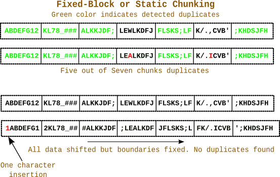The diagram shows insertion, but the same thing can happen for deletion. In general with static chunking duplicate detection is lost after the point where insertion or deletion has taken place.

In order to deal with this, most dedupe solutions use content defined chunking that mark cut points based on patterns in the data. So if the data patterns shift the cut points also shift with them. The diagram below illustrates.

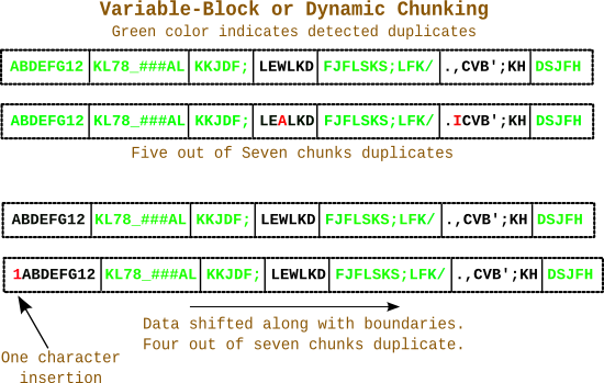The chunks are split based on patterns in data so they are of variable length (but average size is close to the desired length). Since the chunk boundaries shift along with the data patterns, duplicates are still found. Only the modified chunks are unique.

The Rolling Hash computation

Now the question comes as to what data patterns to look out for when determining the chunk boundaries or cut points? The common technique is to compute a hash value of a few consecutive bytes at every byte position in the data stream. If the hash value matches a certain predefined pattern we can declare a chunk boundary at that position. To do this computation efficiently a technique called the rolling hash was devised. It uses a sliding window that scans over the data bytes and provides a hash value at each point. The hash value at position I can be cheaply computed from the hash at position I-1. In other words where ‘n’ is the window size and represents the window bytes at byte position ‘i’. In mathematical terms this is a recurrence relation. Rolling hashes have been used in contexts like Rabin-Karp substring search and Rsync. Today they are used extensively in chunk splitting in the context of data deduplication.

One of the common rolling hashes used in Data Deduplication is Rabin Fingerprinting devised originally by Turing award winner Michael O. Rabin in his seminal paper titled “Fingerprinting By Random Polynomials“. The mathematically inclined will enjoy reading it. There are other rolling hash techniques such as the one used in Rsync, the TTTD algorithm devised by HP, the FBC algorithm etc.

While I am not so much of a mathematically inclined person I still needed a good rolling hash in order to do content defined chunking in Pcompress. After looking at various implementations like the one in LBFS and few other open-source software like n-gram hashing, I came up with an approach that worked well and produced average chunk sizes close to the desired value.

I used a small sliding window of 16 bytes that produces a 64-bit fingerprint at each byte position requiring an addition, subtraction, multiplication and conditionally an XOR for each byte position. It would declare a chunk boundary if the bottom Y bits of the fingerprint were zero. The value of Y would depend on the average chunk size desired. For example for 4KB average size one would look for bottom 12 bits to be zero. The core of the approach is derived from Rabin Fingerprinting. A good description is here: http://www.infoarena.ro/blog/rolling-hash. The hashing approach is a multiplicative scheme of the form:

Where inbyte is Incoming byte into sliding window head, outbyte is outgoing byte from sliding window tail and . The PRIME number I am using is the same value used by Bulat Ziganishin in his SREP tool. Experimentation showed it to produce good results. In addition to this I precompute a table using the irreducible polynomial (represented in GF(2)) from LBFS. The outbyte is used to index the table and the value is XOR-ed with the hash value to produce the final fingerprint. I did some analysis of the chunking approach which is documented in two earlier posts. The results were good.

• Inside Content-Defined Chunking in Pcompress, part – 1
• Inside Content-Defined Chunking in Pcompress, part – 2

A window size of only 16 bytes will raise some eyebrows as typically much larger windows are used. LBFS for example used a 48-byte window and others have used even larger windows. However in practice, as is evident from the above analysis, this implementation does produce good results and the window size of 16 bytes allows an optimization as we will see below.

Optimizations

While addition, multiplication are extremely fast on modern processors, performance overheads remained. Even though I was using a small window of 16 bytes it still required performing computations over the entire series of bytes in order to find cut points. It is very much computationally expensive compared to the simple splitting of data into fixed-size chunks. A couple of optimizations are immediately apparent from the above hash formula:

• Since we are dealing with bytes it is possible to pre-compute a table for
• The MODULUS operation can be replaced with masking if it is a power of 2.

This gives some gains however the overhead of scanning the data and constantly updating a sliding window in memory remains. Eventually I implemented a couple of key new optimizations in Pcompress that made a significant difference:

• Since the sliding window is just 16 bytes it is possible to keep it entirely in a 128-bit SSE register.
• Since we have minimum and maximum limits for chunk sizes, it is possible to skip minlength – small constant bytes after a breakpoint is found and then start scanning. This provides for a significant improvement in performance by avoiding scanning majority of the data stream.

Experimentation with different types of data shows that the second optimization results in scanning only 28% to 40% of the data. The remaining data are just skipped. The minimum and maximum limits are used to retain a distribution of chunk sizes close to the average. Since rolling hash cut points below the minimum size are ignored it does not make sense to scan that data.

All these optimizations combined provide an average chunking throughput of 530 MB/s per core on my 2nd generation Core i5 running at 2.2 GHz. Of course faster, more recent processors will produce better results. The throughput also depends on the nature of the data. If the data has a very specific pattern that causes more large chunks to be produced the performance degrades (Think why this should be the case). This brings us to the worst case behaviour.

Worst Case performance profile

The worst case performance profile of the optimized chunking approach happens when all chunks produced are of the maximum size. That is the data is such that no breakpoints are produced resulting in a degeneration to the fixed block chunking behaviour at max chunksize of 64KB and at the cost of rolling hash computation overhead. In this case the majority of the data is scanned and computed, but how much ?

If we assume minimum chunk size of 3KB, maximum 64KB and 100MB data we will have chunks (considering worst case all max-length chunks). For every chunk of data will be skipped. In my current implementation the value of small constant is 256, though it can be smaller. So the actual skipped size is bytes. In total the number of skipped bytes will be bytes out of 100MB data. In percentage terms it is . In other words 95% of the data will be scanned degrading the performance by more than half.

Now the question is what kind of data will produce this worst case behaviour? If you have seen the rolling hash computation details in Pcompress above, the eventual fingerprint is computed via an XOR with a polynomial computation result from a table. Those values are non-zero and we check for breakpoints based on bottom 12 bits of the fingerprint being zero. So if the computed hash is zero the XOR will set the bits and bottom 12 bits will become non-zero. The hash will be zero if the data is zero. That is if we have a file of only zero bytes we will hit the worst case.

I created a zero byte file and tested this and got a throughput of 200 MB/s and all chunks of the max 64KB length. In real datasets zero byte regions can happen, however very large entirely zero byte files are uncommon, at least to my knowledge. One place having zero byte regions is VMDK/VDI files. So I tested on a virtual harddisk file of a Fedora 18 installation in VirtualBox and still got a majority of 4KB chunks but with a small peak at 64KB. The throughput was 490 MB/s with approx 41% of the data being scanned. So even a virtual harddisk file will have non-zero bytes inside like formatting markers. It is rare to get 100s of megabytes of files with only zero bytes. Finally from an overall deduplication perspective such files will be deduplicated maximally with almost 98% data reduction and final compression stage will also be extremely fast (only zero bytes). So even though chunking suffers, overall deduplication will be fast.

Footnote

If you are interested to look at the implementation in Pcompress, it is here: https://github.com/moinakg/pcompress/blob/master/rabin/rabin_dedup.c#L598

Pcompress updated to 1.1

I just put out a new release that implements proper HMAC computation as described in my previous post. I added a bunch of new tests that test error conditions and error handling for out of range parameters and corrupted archives. These tests caused problems to show up that went unnoticed earlier. These were mostly improper error handling situations. As you see testing may be boring but is absolutely necessary.

I also optimized the use of Zlib by switching to raw Zlib streams. Normal Zlib puts a header and computes an Adler32 checksum among other things. However Pcompress adds its own headers and computes cryptographic checksums like SHA and SKEIN which are light years ahead of the simple Adler32 in terms of data integrity verification. So the Adler32 computation overhead was unnecessary.

I had also tweaked the rolling hash used for deduplication while doing the chunking analysis. This produces better results and improved identity dedupe reduction. Finally I also added header checksums in plain non-crypto mode.

 

Related articles

• Authenticated Encryption and Pcompress (moinakg.wordpress.com)
• Inside Content-Defined chunking in Pcompress (moinakg.wordpress.com)
• Inside Content Defined Chunking in Pcompress – Part 2 (moinakg.wordpress.com)

Inside Content Defined Chunking in Pcompress – Part 2

After cooling off in the hills for a few days, curiosity got the better of me. I discussed in my previous post on chunk size distribution from the rolling hash algorithm that there is a potential trend that can be inferred. Regions having greater variability produce more smaller chunks while regions of uniformity produce fewer larger ones.

I wanted to do some more analysis to see whether there is indeed a trend, short of looking at actual data samples. A trend or correlation will indicate that the rolling hash fingerprint based chunking algorithm is working nicely with desirable properties. Now the question comes how do we define uniformity or conversely variability of data ? I considered two ways of looking at it:

1. Spans or run-lengths of identical bytes values. Fewer longer spans will indicate low variability and vice versa.
2. Zones where same pattern repeats. That is uniform repeating patterns.

Now point #2 is not suitable for our case since repeating patterns can generate repeating break-points in the rolling hash giving rise to many small chunks depending on the repeating pattern size. So from the point of view of our rolling hash this is a form of repeating variability rather than uniformity. This leaves point #1. Long spans of identical byte values will have less chance of triggering break-points since we check for a few least significant bits being zero as our break-point. Spans of zero will of course trigger many break-points but we can ignore that for this analysis as our dataset is quite varied.

I used an initial 24GB portion of the earlier 360GB dataset since I will generating a large number of data points. This initial portion also contains a wide variety of textual, binary (Linux and Windows) and media files. I decided to split the data into 1MB segments and chunk them with an average of 4KB chunk size. I also computed the following properties per segment (of course in a single thread):

• Variability Index
• Ratio of  Total size of small chunks : Total segment size (in bytes)
• Ratio of  Total size of large chunks : Total segment size (in bytes)

Where the following hold:

I somewhat arbitrarily chose the partition value of 16KB keeping in mind average chunk size of 4KB. Eventually all the three values above are ratios and can be directly compared. I also computed the average chunk size per segment and plotted it separately.

Chunk Size Distribution vs Data Variability

Splitting approx 24GB of data in to approx 1MB sized segments produced more than 23400 data items. The chunking algorithm in Pcompress splits segments at a rabin chunk boundary so that every segment gets a set of complete content-defined chunks. This causes a slightly variable segment size.

Since the number of points is very large the lines in the line graph merge together and look like an area graph. Looking at the graphs for a few moments yields the view that there is indeed a correlation between data variability and chunk size distribution. Regions of higher variability do indeed tend to produce smaller chunks and vice versa. Now lets zoom into the middle interesting portion of the Distribution graph to see some more detail (more than 11000 points):

The correlation between the three lines is more clearly visible here but it is not a 100% fit, but then, is anything perfect in life and this universe ? So our requirement of greater data variability producing smaller chunks and vice versa holds in general but does not hold all the time. We can do some quick statistical analysis to get a better idea. First thing to do is to add a couple of polynomial trend lines.

We can clearly see that total size of large chunks is inversely proportional to the data variability with a high degree of probability. This is exactly what we desire. So over a large amount of data localized variations even out and general trends are observed. Finally I also computed Pearson’s correlation coefficients:

So combined with these values and all the previous analysis we can say that clearly there exists a strong correlation of the form which is desirable. Pcompress appears to have a good chunking algorithm unless, of course, someone more experienced than me in this aspect points out shortcomings or mistakes.