Subwoofer isolation pads – Do they make any sense?

In my previous article on my experiments with my hybrid Sonos setup I alluded to trying out isolation pads for subwoofers. These are typically a dense foam base which has a soft fabric covered plywood sheet on the top to hold the subwoofer. The idea is to absorb speaker vibrations and prevent them from transferring into the floor and causing resonances.

Question is do they make any sense or are just snake oil just like so many other stuff in the audio world. The only way for me to determine this was to get a couple of these, test and measure and return if they made no difference. So, did they make a difference for me eventually? Yes, I am keeping those. Should you get one ? It depends!

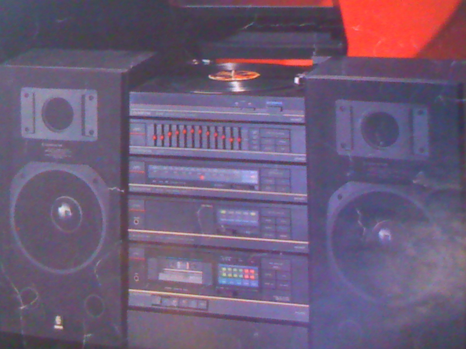
In my hybrid Sonos setup I have two Subs. One a Sonos Sub and another an OSD Trevoce 10” Sub carefully DSP tuned to complement the Sonos sub. Even after lots of tweaking of settings and DSP, furniture and speaker adjustments there was a slight nagging boominess to the bass. Costly room treatments were not an option, especially in a rented apartment. After researching a bit, I ordered two Auralex Subdude II isolation pads which subjectively, made the boominess disappear with tighter bass. However, I wanted to measure with REW. REW is not subject to placebo effects so I hoped to get an objective picture.

Note here that the Sonos Sub has two opposing force-canceling drivers resulting in negligible vibration of the subwoofer cabinet but some energy still transfers to the floor from direct contact. The OSD Sub has passive radiators but they are not force-canceling, so it does vibrate. Note also that I have a carpeted floor so carpet should absorb some vibrations from the subs. I was interested in the Decay graphs from REW to understand the extent of resonance/ringing per frequency range. I decided to use the spectrogram graph type as it shows decay times independent of peak volume levels. My measurements were all volume matched to 75Db SPL for Pink Noise. The spectrogram is a view of the waterfall 3D graph from above.

I took two measurements, one without the Auralex pads on both subs and one with them. My first measurements showed reduced decay times, albeit small, but across the entire frequency range! This was very surprising to me. I was only tweaking the subwoofer setup, so how can it impact the higher frequencies. I could not believe those results and was confused. I could not clearly recollect if I had done something odd or maybe even changed the settings in the middle, or it could be differing background noise. So, I used the setup for a few days and took another measurement on another day at a time when things were uber-quiet and there was only me at home. I took two measurements in quick succession with and without the pads and was very careful to not affect anything and ensured background noise was minimum. I got the same result! So, I measured yet again and once again got the same result!

The following is a spectrogram overlay that compares the decay times. Click on the image for a bigger clearer picture. All measurements were taken from the Main Listening Position or MLP for short. I used a UMIK-1 and it was pointing straight. I did not use the 90 degree config. I will try that another day. Maybe, it will pick up the reflected sound better and show a bigger difference.

Spectrogram boundary in white = measurement without Auralex pads. Inner rainbow colored spectrogram = measurement with the pads.

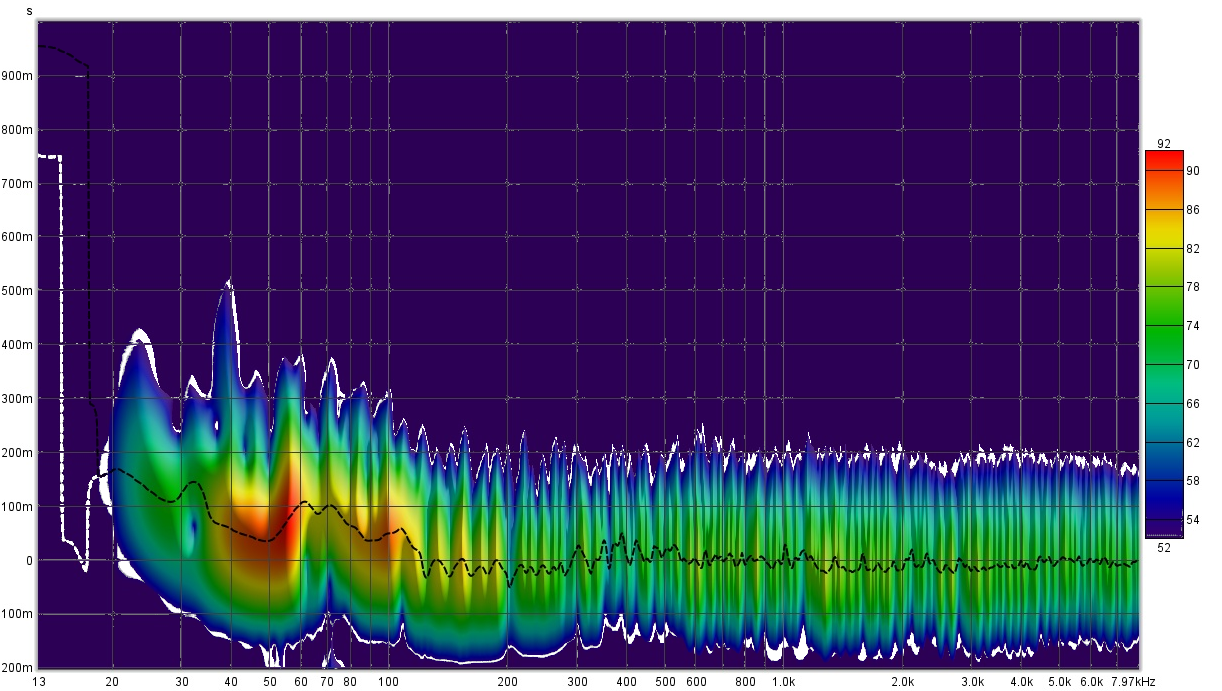
The vertical axis is decay time. It is clear that the inner spectrogram has smaller decay times across the frequency response. The benefit is small, but it is present even with my carpeted floor and subjectively audible. Human hearing is very sensitive to timing changes, reverb, echoes etc. So how is this working? I suspect a few things:

• The Auralex are doing their job at the lower frequencies.
• REW does a frequency sweep so, I suspect the previous frequency’s decaying tone is affecting the next in the range. But this still does not explain the benefit at the higher frequencies much beyond the time of the lower frequency decays.
• I live in an apartment, on the second floor and the building is made of wood and synthetics (drywall for eg). There is no concrete. So vibrations, even minor ones are transmitted easily.
• The subwoofers are kept just next to my bookshelf speaker stands that have metal spikes into the carpet. So, the isolation pad foam are likely absorbing higher-frequency vibrations through the carpet transmitted to the floor via the stand.

So, finally the question, should you get an isolation pad? Considering the following questions can help:

• Do you live in an apartment? If yes then it can make some sense to avoid trouble with your neighbors.
• Is the building made of concrete or wood? Obviously it makes more sense in a wooden construction.
• Even in a concrete building do you have a wooden floor?
• Do you have a carpet? Wooden floor with no carpet and it makes more sense to get an isolation pad for your sub.
• Are you living in your own house, possibly concrete construction and have a carpet with audio setup on the ground floor? Though it will make hardly any difference to the sound, you can still get one for mental peace, especially if you have OCD like me!!
• Do you have room treatments like acoustic panels and bass traps? Please still buy these isolation pads because they are another fancy item to talk about and show off your deep knowledge of room acoustics to friends and family…

Caveats

Well, the last two jokes apart, there is some sense in getting these pads based on your situation as is clear from the remaining points and the earlier discussion. However, one thing I could not measure is how much floor and wall vibrations were present before and after. Measuring that accurately with enough sensitivity requires expensive equipment. The free smartphone based apps are likely not sufficient here. Subjectively, listening to music from outside my apartment, the low frequency effects did sound lower at the same volume. Also, my measurement microphone was horizontal, pointed towards the speakers. I later learned that it is recommended to point it upwards and use the 90 degree calibration file to better assess room effects.

Boot Environments on Linux

I have been busy working on a bunch of exciting tech last few years with very little time for anything else apart from family. The typical startup grind. However, better late than never, I found a bit of opportunity to write up on something I have been hacking on (along with couple of others) and have been put out in open-source.

We have seen the concept of Boot Environments initially with ZFS on Solaris. Because the filesystem supports snapshotting and cloning, it is possible to create another virtual copy of the entire root filesystem as a clone of the currently booted root. It is then possible to mount that clone, upgrade packages inside that prefix and finally reboot into the upgraded clone after adding a grub entry for it. There are several advantages of this approach.

• The operation of cloning the filesystem is instantaneous due to the Copy-On-Write design. There is no need to perform a costly copy of the entire root filesystem image.
• During the upgrade the box is up and running and in production use because the currently booted environment remains untouched. The only downtime is when we reboot.
• Since the currently booted environment is untouched the upgrade is very safe. Any failures or breakage during upgrade would mean destroying the clone and starting again from the beginning, in the worst case.
• If we discover issues after booting into the updated clone, we can easily reboot back to the previous working Boot Environment.
• Because of the COW design the upgraded clone only occupies space for the packages that were actually upgraded. Unchanged package content is shared with the parent dataset of the clone. This un-duplication is space efficient.
• It is possible to have multiple boot environments on the box without having to worry about partitioning.
• Because of the pooled storage design all datasets or clones share the same pooled storage space avoiding hard partitioning and fixed space allocation headaches.
• Multiple boot environments are *extremely* useful in a testing and development setup where multiple software releases can reside on the box. To select a certain release for testing or experimenting, just boot into the appropriate BE (Boot Environment). Messing around is also easy. Create another BE from the current one. Boot into it and mess to your heart’s content. The original BE remains safe as long as you do not screw the disk or the bootloader of course!

I can go on some more but lets draw a line here. Now, we wanted to get the same stuff on Linux. It is possible given we have the nice beast called Btrfs. Btrfs, till sometime back has been controversial and criticised quite a bit. However, I noticed that it has been maturing of late. Number of serious issues have gone to negligible. Many fixes and improvements have come. All of the rants I found via Google were at least couple of years back and mostly were older than that. This gave us the confidence to start testing it and eventually use it in the products my employer sells. We did have to go through a learning curve getting to grips with the nitty gritties and idiosyncracies of Btrfs. It created a bit of initial teething troubles and deployment issues but it was manageable.

I looked around to see if the BE capability already existed but found none. I came across things like apt-snapshot or Snapper which are similar but not quite the same. Our hard requirement was that upgrade must not touch the running environment. So, in the end, we came up with our own scripts to implement the BE feature.

Since our Linux environment is based off Ubuntu the root subvolume is ‘@’. We then create a writable snapshot of ‘@’ as our initial root subvolume and that becomes our first BE. Subsequent upgrades creates writable snapshots of the current booted subvolume. In addition, the ‘@’ subvolume is always mounted under /.rootbe in our environment and all the BE subvolumes and mounted under it including the currently booted one which is also mounted at ‘/’ obviously.

Btrfs has the concept of a default subvolume, however we do not change that. Rather, we just use the ‘rootflags=subvol=…’ parameter. This allows us to have the primary grub menu in a single place and access always via /.rootbe/boot/grub/grub.cfg.

The entire show is managed via two shell scripts. One to do the BE management (create, delete, list etc.) called ‘beadm’ and one to upgrade the current environment by creating a new BE called ‘pn-apt-get’. Both of them are available at this url: https://github.com/PluribusNetworks/pluribus_linux_userland/tree/master/components/bootenv-tools

The ‘pn-apt-get’ script creates a new BE and runs ‘apt-get dist-upgrade’ inside a chroot. It assumes that the ‘sources.list’ has been setup properly.

In addition to all this I wanted to optimize the space used by having dpkg Not replace files in a package being upgraded if the new file is identical to the one already installed. I needed to add a small Dpkg patch to achieve this: https://github.com/PluribusNetworks/pluribus_linux_userland/blob/master/components/dpkg-ubuntu/debian/patches/skip_unchanged.patch

All this allows us to do safe, fast, in-production upgrades and only incur downtime during the reboot.  One quirk I had to deal with was BE space usage reporting. I had to turn on the ‘quota’ feature of Btrfs to get accurate space accounting even though I do not use quotas in practice. This also meant that I hit a couple of obscure quota bugs (especially after subvolume delete) in the 4.4 Ubuntu Xenial kernel release that we have been using (logistics issues). To work around I found it sufficient to do a periodic “quota rescan” every few hours.

Pulling out Libarchive metadata

I use a Libarchive copy in Pcompress to do archiving. Pcompress prepares the list of pathnames to be archived and calls low-level libarchive apis to archive the pathnames for fine-granied control. For example, the pathnames are sorted via fairly involved heuristics. The output from Libarchive is passed to the compressor stage. In addition, a few file type specific filters are used prior to writing file data via Libarchive apis.

The libarchive output stream is split into buffers and compressed in parallel, the basic approach in Pcompress. This results in a solid compression mode that achieves a high compression ratio. However this also has a few problems:

1. Libarchive does streaming archives so archive metadata is inline within the data stream. This causes breaks within the actual data stream and pollutes the context eventually reducing compression ratio slightly.
2. Simply listing the archive members, without actually extracting them to disk requires decompressing all of the data.
3. Similarly extracting a single member means decompressing everything before it (which is the problem with things like tar.gz anyway).

So separating out data and metadata would be beneficial. Metadata can be kept in a separate compressed stream from the data which would allow fast access in the couple of use cases above. To achieve  this, Libarchive would need to indicate to the client callbacks the type of request: data or metadata. This is tricky. The model of Libarchive is to just request some data as in:

1. When extracting it invokes the callback. The callback returns a blob of data and tells it’s length. When Libarchive has consumed all of the blob it requests for more.
2. When archiving it invokes the callback to with a block of data to write with a specified length.

There is no differentiation between data and metadata as the formats are typically streaming formats. Pcompress uses PAX. The immediate thought that arises is to have Libarchive indicate via a flag in the archive structure whether the request is for data or metadata. This works fine when archiving, since blocks of data and metadata are written separately. The client callback can use an api call using the archive structure to determine whether data or metadata is being written. The trouble arises during extraction

This simple technique of using a flag within Libarchive is not sufficient when extracting an archive. Looking into the archive_read code, one can notice that there is a filter structure, that keeps track of the current buffer passed from the client callback and the internal cache to implement a virtually zero-copy architecture. The filter structures can be cascaded if there are multiple filters in the chain. The root filter is obviously the NONE filter. See archive_read_open1() in archive_read.c. Once all data in the client buffer is consumed, the callback is invoked again to request for more. So, If data and metadata is stored separately, then the client callback will have to stitch them together and re-create the original archive stream which has to be passed back to Libarchive. This is complicated and very expensive in practice. In particular, the buffer copying required would defeat Libarchive’s zero-copy approach. Eventually, the solution I landed upon, is to introduce a secondary filter structure accompanying each normal filter struct. I call this the shadow filter. This is identical to the main filter struct and is only initialized in case metadata streaming is being done. Now, Libarchive can use this shadow filter structure to keep track of the separate metadata stream. Whenever a metadata request is made the client can return a metadata buffer which is tagged onto the shadow filter. Data requests are handled via the normal filter structure.

The changes needed in Libarchive to get this working were, in fact, smaller than I anticipated and are all inside the Libarchive copy in Pcompress trunk(changeset 1, changeset 2). A couple of obvious new api calls are needed: archive_set_metadata_streaming() and archive_request_is_metadata().

The current Pcompress trunk packs metadata into 3MB chunks and marks them as metadata chunks. These chunks are compressed using the Delta2 filter and Bzip2 compression. During extraction, it opens two handles to the archive file. One handle is used by the metadata thread to read metadata chunks and skip data chunks while the main thread does vice versa. This of course precludes pipe-mode streaming operation.

Currently, listing of archive contents is extremely fast as Pcompress has to just decompress the metadata chunks and return that to Libarchive. The data sections are simply skipped. I am still working on a mechanism to do optimized selective extraction. For this I will have to store additional metadata to indicate which data chunk holds the start of the file contents so that the data decompression thread can quickly skip forward to that one.

So what’s the difference in terms of compression ratio and timings, with and without metadata streaming? Using the 10GB compression benchmark from Matt Mahoney here’s the results (83435 archive members) on a MacBook Pro late 2013 model:

1. Metadata Streaming:
   • pcompress -a -l14 -s60m -t5 10gb 10gb.pz  —> archive size: 2936436327 bytes
2. Without metadata streaming (notice the -T flag):
   • pcompress -a -l14 -s60m -t5 -T 10gb 10gb.pz  —> archive size: 2939247636 bytes
3. Time to list archive contents with metadata stream:
   • ./pcompress -i 10gb.pz  0.90s user 0.10s system 84% cpu 1.184 total
4. Time to list archive contents without metadata stream:
   • ./pcompress -i 10gb.pz  1106.16s user 28.63s system 346% cpu 5:27.38 total

So compression done using inline metadata (without metadata streaming) is about 2.6MB or 0.1% larger. It is a small amount given the archive size, but a difference nevertheless. Larger relative benefits will be visible for archives having a large number of small files. However the real massive benefit is seen in the total time to list archive contents. 1.2 seconds vs 5.5 minutes: It really is a no-brainer.

Scaling Deduplication in Pcompress – Petascale in RAM

My core objectives with Deduplication experiments in Pcompress has been to achieve large-scale data handling capability using tiny chunks (4KB and even 2KB). This has traditionally been extremely difficult to the point of being nearly impractical. The algorithms in Pcompress can now achieve this without loss of performance, at least for archival data streams. Read on to find out more.

Approach

I have in the past alluded to a an indexing algorithm in Pcompress that allows me to deduplicate large data using only a tiny memory-resident index. I finally found some time to write about it. The basic idea is quite simple and is not entirely new. What is new, is the way certain components of the approach are implemented. The steps are simple:

1. Break dataset into large segments, such that each segment is a collection of adjacent variable-length chunks as derived using a chunking algorithm.
2. For each segment create a chunk-list file on disk which contains the list of chunk hashes.
3. For each segment compute one or more similarity identifiers and store in an index.
4. If one or more similarity identifiers for two segments match then we know that the segments have at least a few chunks in common. In that case load the chunk lists of the segments from disk and deduplicate the chunks.

If the segments are large enough then a relatively tiny similarity index can address large amounts of data. This scheme requires one disk read per bunch of chunks reducing lookup and access times. Also each chunk list is one file and is read sequentially improving read times. The chunk list files can also be stored on SSDs to speed up even more. The similarity index can be a RAM-resident hashtable giving the fastest possible lookup times. Since each segment is a collection of chunks, I experimented using different chunk counts and found excellent results having 2048 chunks per segment. Thus the segment size is of variable length. For an average chunk size of 4KB we get 8MB segments on average, for 8KB chunks we get 16MB segments and so on.

Many Similarity based Deduplication approaches use files as the objects for checking similarity. However this suffers from a problem that very large files can give rise to loss of accuracy and poor deduplication ratio. Conversely too many tiny files can bloat the similarity index. The approach described above avoids these extremes. A somewhat similar approach has been described in the SiLo scheme.

The old guard – MinHash

The effectiveness of the approach described above hinges on the effectiveness of the similarity indexing scheme. Here I based my implementation on the good old MinHash technique. This technique has been used commonly in data mining and web search to determine similar documents, detect plagiarism, perform clustering and so on.

Essentially we break up a document into a set of semantic pieces, compute multiple hashes per piece and identify a subset of pieces that possess the numerically lowest hash values. If such k-min subsets of two documents match then we can say that the documents are somewhat similar to each other. In this deduplication use case a document is nothing but a segment. Since each segment is a set of chunks, each sematic piece is a chunk as determined by the chunking algorithm. The question is what hashes to compute for each chunk in order to apply the MinHash algorithm? (See MinHash for Dummies for a layman’s explanation of MinHash).

After lots of experimentation and head scratching it turns out that the cryptographic hashes computed per chunk can themselves be used via truncating. Truncated cryptographic hashes are themselves independent hashes. I took this idea to its logical extreme and split each cryptographic hash into a set of smaller hashes. These can be thought of as the permutations of the hash function. Then I can sort these hashes numerically and select the K lowest values to get my K-min-values sketch. If one or more elements of the KMV sketches of two segments match then the segments are deemed to have at least a few chunks in common. How small to truncate a hash? It turns out that 64-bit hashes provide a good approximation. So if we are using, say SHA-256, then we get 4 smaller hashes from each chunk hash. These are then numerically sorted and the 20 lowest unique values are chosen. Pictorially this approach can be depicted as below.

The number 20 and other thresholds were arrived at experimentally, to give a good balance of memory usage vs deduplication effectiveness. Increasing beyond 20 hashes, results in diminishing returns on dedupe effectiveness while linearly increasing memory consumption. The point of inflection actually comes at 16 hashes, below which, dedupe effectiveness falls rapidly. The chart below shows the results of testing on a 360GB dataset that I have used in previous occasions.

Here .

The interesting thing here is that this approach results in high deduplication effectiveness to the extent of 90% to 95% of the effectiveness of straight forward exact dedupe using a simple chunk index. The choice of the hash function (SHA2, SHA3, BLAKE2 etc) has little bearing on the outcome. Here is another chart showing a comparison of this similarity based deduplication (using various datasets and hash funtions) with the exact deduplication baseline.

Memory Usage

Lets consider the case of 4KB average chunk size. Each segment contains 2048 (approx) chunks, which gives us 8MB average segment size. For each chunk we derive a 256-bit crypto hash which results in 4 64-bit similarity hashes per chunk. We select the lowest valued 20 unique hashes per segment which form the similarity indicators. So we need 160 bytes of similarity indicators per segment. In addition to this we need to store 64-bit pointers to the actual segment data on disk. The segment data is basically the chunk hash and data pointer list stored on disk. So the storage requirement is doubled to 320 bytes. The similarity indicators for a segment are kept in a hash table. So we need to consider some data structure overheads as well. Assuming 4 bytes of overhead on average we have a final storage requirement of 400 bytes per segment.

Now assuming 8MB segment size and one Petabyte of 100% random data where no duplicates exist (worst case), we would need 134217728 segments. This translates to 50GB of worst case memory usage. If we use 8KB chunk size, then the calculations lead to 25GB RAM requirement for the worst case. These memory values are not too much by present day standards and typically data will have duplicates. So RAM requirement will come down by the extent of duplicates present, especially when using the deduplicating storage architecture I had described earlier. If we limit data handling to say 500TB, then even smaller 2KB chunks can be used. These are practical resource limitations. The algorithm does not have any inherent limitations. If we use a well-endowed server with say 256GB or more of RAM then petascale data can be handled using 2KB chunks as well. Performance will be lower of course.

To the best of my knowledge there is as yet no dedupe product that can handle a petabyte of data using small 4KB chunks and an in-memory index. I may be wrong, so please add comments if you know of another such system. If you are looking at less than a Petabyte then even 2KB chunks are possible – virtually no one does this today.

This indexing scheme is actually implemented in Pcompress today and works quite well. It can actually reach raw a dedupe processing throughput of upto 500MB/s (discounting I/O) on my average laptop. Of course there are many other optimizations both algorithmic and architectural some of which I have posted about earlier. I am presently working on the persistent similarity index part which would allow creating versioned incremental archives.

Related Posts

• Efficient Deduplication is all about Tables – Yes so true but Permabit Albireo is still talks about large 64KB chunks.
• Architecture for a Deduplicated Archival Store Part 1.
• Architecture for a Deduplicated Archival Store Part 2.

Getting into the Groove

I’m an audioholic, by birth. My ears tend to be analytical of the sound it is hearing. So I simply lose interest in music unless I’m in a real concert or the audio is being reproduced by a good system. A small stereo system or even the typical consumer Home Theater in a Box setup would not satisfy me. I’d rather not listen to music at all if those are the only sound sources that I could get.

My dad was like that as well. in my early years I grew up listening to a Sonodyne Uranus hand-equalized by my dad. That was the best he could afford at that time and it was a decent beast. It came with a dual cassette deck, an AM/FM Tuner, a discrete 12-band graphic equalizer and an integrated pre-power amp with the output stage driven by two STK 4131 II power mosfets. It also had an optional turntable which we did not go for. There were 2-way ported (bass – reflex) stereo speakers which could handle 50W RMS each. However the mosfets could only deliver 20W RMS per channel. At that day and age it was good enough for us. Stereo nirvana in fact. I plugged in a CD player much later.

After enjoying with that for more than 8 years we had to dispose of it. It had aged and required constant maintenance. Then many life changes happened to me and I could not get my hands on a decent setup, for one reason or the other that would also include lack of budget at the right time. Finally moving into a new house provided the right opportunity. Luckily I managed to allocate some surplus funds. In addition my timing was just right to land a deal with the 3-day ProFx anniversary sale. A 25% discount on the package plus freebies. This is what I grabbed:

1. KEF Q-series 5.1 spkr system: Q700 Floorstanders, Q200c Center Channel, Q400b Sub and Q800ds dipole surrounds.
2. Denon AVR 2313 receiver.
3. 33M speaker cable free gift box.
4. Free installation.
5. A pair of Denon Urban Raver earphones via a lucky draw.

I already have a PS3 as my primary media player which I readily hooked onto the AVR. The discount and the effective market price of the KEFs in India meant that I paid for the speakers and got the Denon for peanuts. Yes the AVR 2131 model has been phased out and replaced with the new AVRX series. However Denon, with AVRX, has actually consolidated it’s lineup and reduced the wide range of models on offer to reduce customer confusion along with a few technical improvements. So I did not lose much by going with an older model. In fact who cares when I get it for peanuts. The Denon comes with this awesome Audyssey MultiEQ XT feature which can compensate (equalize) for room imperfections to a good extent.

As I mentioned before, I’m an audioholic but not an excruciatingly technical one. I’d not get into aspects of acoustical engineering to setup this system in my living room. I just wanted something that would sound good to me. Whether it is a good measured audio frequency response or not I’d not really bother (though I’d be curious to find out). As usual, the installer did a basic setup and did not spend too much time. There were several problems with the installation and the room:

1. The floorstanders were too close to the walls. Possibly because he was trying to match speaker separation to listening distance and get an equilateral triangle for good imaging. I wanted to avoid wall reflections and compromise a bit on imaging.
2. The room is rectangular with 9’1” height, 11’2” width and 16’2” length. The listening position is lengthwise. So keeping the floorstanders away from the walls meant I could only get an isoceles triangle with respect to the listening position. Moving the rear sofa forward would upset the room decor and badly upset the entire family!
3. I have a coffee table made of pre-laminated particle board.
4. The Sub’s volume was at 80% and not the recommended 50%.
5. The Sub’s crossover knob was set at 80Hz while recommendation is to set it at max (150Hz) and let the AVR decide on the exact crossover values.
6. I made him run Audyssey but the environment was bad: Some nearby drill machine came on at the wrong time, a dog barked, neighbour’s car went past arrgh!
7. He did not have a MIC stand with boom. So he placed the Audyssey MIC on the sofa back to do measurements which is crap.
8. My room has walls on 3 sides the back of the listening side is open with a stariway, followed by dining and kitchen space.
9. Seen from the listening side, the left side wall ends 3.5ft shorter than the right side wall to allow walking space and access to a guest bedroom.
10. My TV is a Sony 37-in, HD-ready, flat panel, 6 yrs old. I do not have the budget to go in for a new TV at this time.

In addition to this the room has wooden look flooring made of MDF. The MDF boards rest on two layers of foam which in turn rests on the concrete floor below. Since the floor is not hardwood and it rests on foam, I decided not to go for mats in front of the floorstanders. The coffee table rested on a central carpet in any case.

Initially the sound lacked depth and the bass was missing. I do not like boomy bass but the earth-shattering explosion in Skyline seemed like a tinny Diwali firecracker. Dialogues were too loud. Floorstanders seemed to do a lot of work at the low end leaving the sub idle. Treble seemed analytical. Lastly the sound imaging seemed to be converging at a point a couple of feet above my head!

Eventually it took me a month of playing with speaker positioning and Audyssey and a wild goose chase due to a HDMI weirdness on my old TV to finally get something I like really like listening to. Some aspects of my adventure in summary are below:

1. Move floorstanders away from wall by upto 2’1”. Move subwoofer from left to right. Left side was being blocked by the larger sofa impairing the subwoofer’s bass.
2. Cover the darned, but aesthetically and practically required coffee table with a mat to absorb reflections. Looks good as well.
3. Fix the dipole surrounds to the side walls with screws and two small aluminium brackets. They are not exactly aligned due to the different wall lengths. I could not place them at the rear, on stands, due to aesthetic and practical problems. One of the speakers will then come within the common walking area and if children bump into it, my hard-earned money goes down the drain!
4. The right side wall has a large window with two – layered curtains which prevents reflections. The right wall was empty, so I placed a decorative grid-design shelf in the middle. Looks good and diffuses reflections somewhat.
5. Build a boom stand for the Audyssey MIC with some leftover MDF pieces from my modular furniture construction. This kind of a MIC stand is generally considered not good but I did some improvising to get fairly good results.
   • I made the stand short (about 27” tall) and rested it on the sofa, rather than the ground to avoid transmitting vibrations from the ground to the MIC.
   • I set the ear level height to 23”.
   • Covered the base plank of the stand with sofa cushions during measurement to avoid unwanted reflections.
6. I did the Audyssey measurements during midnight 1AM so there will be pin-drop silence. The only sound is from an UPS fan.
7. I followed the following guide, though not down to the letter: http://www.hometheatershack.com/forums/audio-processing/68407-audyssey-multeq-faq-setup-guide.html
8. I had to re-run Audyssey about five times as I kept making small mistakes, tweaking the speaker placements and trying a couple of MIC patterns. Five times being a night owl, much to the consternation of my wife and being groggy at office the next day.
9. I noted down the furniture positioning measurements. This is so that when the furniture is moved for cleaning I can recreate the exact layout that was used to run Audyssey, accurate to the inch.
10. The HDMI Control (CEC) would not work reliably with my old Sony Bravia. This would result in sound only coming from the TV, not the KEFs!! Imagine my frustration playing movies and music on the PS3 with the expensive KEFs sitting and watching idly. It would work intermittently. I tried to change HDMI cables, update firmware on PS3 and the Denon, reset settings to no avail. After a wild cursing chase I managed to figure this out. Turning off HDMI control fixed the problem. It however, prevented automatic HDMI switching from the DTH set-top box to TV when the AVR is switched off. Luckily my set-top box has component video and stereo audio out which I could directly connect to equivalent inputs on the TV. In any case component video is more than enough for the family to watch standard-definition TV channels. If I want to watch something like NatGeo HD I’d switch on the AVR.
11. I want to add front height speakers later on, so did not go for bi-amping the fronts. I know I’d have to re-run Audyssey … arrgh.
12. I set the front crossover points to 60Hz for the front towers and 80Hz for the center. Audyssey had set them all to 40Hz.
13. Increased the Subwoofer level from -0.5db to 0db.
14. I switched off Dynamic EQ and Dynamic Volume.

Finally, after all this circus, I have something that I look forward to listen to and watch. The great thing is that the last Audyssey round was just perfect for my ears that I do not have to mess with the tone control or the speaker levels(except for the slight sub tweak). All I did was to increase the Dialogue level a bit while watching Ender’s Game. Turning up the volume while watching the explosion in Skyline makes one look around to ensure that it is not his living room items that are breaking.

Stereo music sounds equally good with deep thudding, not booming bass and clear treble. The imaging could be better but is not too bad either. I cannot change my living room! Boney-M and the Love At First Sight CD just come to life. Sultans of Swing is smooth. All the instruments in Classic Rock are rendered crystal clear; I can make them out. Kishore Kumar and Hemant Kumar seem sitting right in front of me! The KEFs are truly glorious.

Distributed Storage and FPGAs

I have been super busy for the last few months getting a new house completed and moving into it. It takes an incredible amount of effort. Me being the DIY type also invested some energy in being hands-on with Carpentry, Masonry, Plumbing, Electricals, Gardening and sundry other stuff, to the consternation of my family and my utter satisfaction and utter exhaustion! Anyway that being settled mostly, I am getting back to catching up on digital stuff.

One of the very interesting developments that caught me, was this post on the Register: http://www.theregister.co.uk/2014/01/31/bluedbm_fpga_storage/. A storage controller on a FPGA linked together with other such controllers on a low-latency bus. How cool that is in terms of distributed storage. From the outside, we get a high-performance distributed storage pool. Obviously flash is also there in the picture. Thinking further on this one can also consider this system acting as a front-end cache for a remote WAN-linked storage archive.

I am wondering, if they can implement some storage controller functionality using a FPGA, can it also be done using CUDA. In that case, we can use something like GPUDirect for low-latency Infiniband access from the GPU. This would avoid having to deal with custom silicon. From yet another perspective, it might be possible to do something similar with the Pluribus Server-Switch built from off-the-shelf components.

Scaling Deduplication – Sepaton’s Big Data Backup appliance

Came across this news piece on Register dated back to October: http://www.theregister.co.uk/2013/10/16/sepatons_superduper_deduper/

Potentially handles upto 16PB of backup storage with Global Deduplication – Great! The performance and features on paper are really top of the line. Beats the competition on most aspects. If I look at the deduplication features a few things look interesting vis-a-vis those that I have put into Pcompress.

It mixes “Hash-based inline deduplication” and “Post-process, content-aware deduplication”. The article is not clear what exactly this means. There are two possibilities. Firstly it can detect duplicate files during ingestion, store only a single copy and then do block-level dedupe as post-process. Secondly it can deduplicate using large chunks during backup ingestion and then dedupe using small blocks as post-process. This is of course to not hurt backup performance and scale to large datasets. Post-process deduplication is a common technique to scale deduplication without affecting I/O throughput of in-flight data. It has also been used effectively in Windows Server 2012 to do primary data deduplication.

Sepaton can do analysis of data types and change rates in data to apply the most efficient dedupe mechanism or even skip dedupe for encrypted and compressed files that virtually do not deduplicate at all.

The other interesting features include byte-level deduplication for databases that store data in block sizes less than 8KB and using flash based SSDs to store the global index. I am not sure what this “byte-level deduplication” exactly means but it appears to be a delta-differencing mechanism. Now the question is how efficient restore can be when delta-differencing is used.

In some of the posts on Pcompress design I have already mentioned about using SSDs for storing all kinds of metadata. Fast metadata access is critical and this is the logical choice. However the other “new aspect in Pcompress is the ability to use small blocks for deduplication without losing performance and giving good scalability“. This is a key feature that most of the current solutions seem to be missing. Pcompress can use blocks (or chunks) as small as 2KB without losing too much performance. With 2KB chunks it can potentially scale to 500TB of 100% random data using a 40GB in-memory global index. If the data has duplicates then the index size becomes smaller. This deduplication occurs with 95% efficiency of a full chunk index based brute-force dedupe. This single capability solves a sticky problem that dedupe solutions has been dealing with for quite some time. The metadata structure that I have discussed in earlier posts also helps with overall performance. The approach is based on similarity detection of large regions in the data stream. The chunks lists of those regions are then sequentially loaded from SSD and compared to perform actual deduplication. The similarity detection technique is simple and novel. It avoids any kind of complicated math, fuzzy hashing etc.I will detail it later.

There are other unique techniques in Pcompress like a partially vectorized rolling hash, scanning less than 30% of the data to locate chunk boundaries, parallelized deduplication and others that contribute to the overall performance. I have posted about a few of these earlier.

In addition to the above, the recent zip-like archiver capabilities that I have added into Pcompress introduce data type detection and automatic selection of filters and compression techniques to suit the data type. However the big missing piece in all this is that Pcompress is still a stand-alone utility. It needs work to turn it into an archival store where data can be ingested incrementally and selective data streams extracted for restore. Also an efficient partitioned indexing is needed to be able to scale deduplication in a cluster without losing deduplication ratio.

Related articles

• Pcompress gets archiving features (moinakg.wordpress.com)
• Storage Myths: Dedupe for Databases (flashdba.com)
• Architecture for a Deduplicated Archival Store: Part 1 (moinakg.wordpress.com)
• Architecture for a Deduplicated Archival Store: Part 2 (moinakg.wordpress.com)
• High Performance Content Defined Chunking (moinakg.wordpress.com)
• Inside Content-Defined chunking in Pcomporess (moinakg.wordpress.com)
• Inside Content-Defined chunking in Pcomporess – Part 2 (moinakg.wordpress.com)

Pcompress gets archiving features

Among a busy personal schedule for the last two months, I have managed to work quite a bit on adding archiving features to Pcompress. Thanks to the excellent LibArchive, Pcompress can now bundle up a bunch of files into a compressed archive. This is a desirable and useful capability that was missing till date.

With the addition of archiving capability Pcompress can now perform advanced detection of file data and tweak its compression behaviour to achieve the best results. Below is a short list of features and behaviour that the github code has as of this writing:

1. Pcompress enumerates the file list to be archived and sorts the files by extension/name and size using an incremental merge sort to minimize memory use. This sorting, groups related files together and clusters small files to achieve the best compression and deduplication behaviour. For example see this paper where a similar technique has been discussed to improve deduplication: https://www.usenix.org/legacy/event/atc11/tech/final_files/Xia.pdf
2. File types are detected via extension and/or file header parsing for magic numbers. Compression buffers are split at boundaries where files change from one type to another to avoid mixing unrelated files in a single compression buffer. It helps to improve compression ratio.
3. More importantly, this file type detection is used to apply data-specific compression techniques more effectively, making the Adaptive modes in Pcompress extremely powerful. The following data specific algorithms are used:
   • LZMA – Most binary data.
   • PPMD – Most Textual data.
   • Libbsc – DNA Sequences, XML/HTML etc, BMP and TIFF images.
   • Dispack – Preprocess 32-bit x86 executable binaries.
   • PackJPG – Reduce JPEG size by upto 40%. This is new lossless JPEG compression technique by Matthias Stirner.
   • Wavpack – Compress WAV files better than any regular compression technique. This is still a work in progress.
   • Detect already compressed files and for some heavily compressed data just use LZ4 to suppress some internal headers and zero padding. This avoids wasting time trying to compress data that is already heavily compressed.
   • There are other data specific filters around like MAFISC which I am looking at.
   • For Dispack, 32-bit x86 executables are detected and the data buffer is then split into 32K blocks. Some approximate instruction statistics are checked to determine whether to Dispack that block.
4. Compression buffers are split either at hash-based or data type change based boundaries improving both compression and deduplication.
5. LibArchive is used as the backend archiving library whose output is passed to the buffering, deduplication and compression stages in a logical pipeline. Synchronization is kept simple by using semaphores. LibArchive runs in a single thread and the data fetch from archiver to compression is also done at a single point. Thus there is exactly one producer and one consumer. This simplifies synchronization.
6. To the extent possible data copying is avoided. LibArchive’s callback routines are used to copy data directly into the compression buffers without resorting to pipes and such.

The filters like Wavpack and PackJPG need to work with LibArchive. However LibArchive does not support using external filter routines so it took a while to work out how to have external file filters pipelined before LibArchive. Note that since Pcompress uses a custom file format and consumes the output of LibArchive, there is no need for strict compatibility with standard archiver formats like Tar, Pax, Cpio etc. LibArchive for its own requirements obviously strives to attain strict conformance allowing no user-defined headers. So one of the big problems was to flag which files have been processed by a custom filter. One easy way was to add an extended attribute programmatically. However LibArchive does not provide a way to delete a single attribute during extraction. There is a call to clear all attributes! One does not want internal, programmatic use attributes to be extracted to disk. I was stuck. Eventually it turned out that I could use contextual inference. A file preprocessor like PackJPG will add its own magic header to the file. Thus during archiving I can look for a JPEG header and only then pass the file through PackJPG. During extraction I can look for the PackJPG header.

However the question comes, what if I have some PackJPG processed files and are archiving them using Pcompress? Won’t it revert to normal JPEG during extraction even though I do not want it to? Well the filename extension is also checked. During archiving, normal JPEGs are filtered but their extension remains as jpg or jpeg. So only files having a Jpeg extension but having a PackJPG header are unpacked during extraction. If you use the standalone PackJPG utility to pack your JPEGs, then will get a .pjg extension which will be untouched by Pcompress filters during extraction. However, truely speaking, LibArchive needs to add a simple xattr deletion function to avoid all this jugglery.

File types during archiving, are detected by a combination of filename extension and magic header inspection. To lookup filename extensions one obviously needs a hashtable. However there is a bit of detail here. I have predefined list of known filename extensions with their corresponding file types, so instead of using a general hash function I needed a perfect hash function. That is, the number of slots in the table is the number of keys and each known key maps to one slot. An unknown key can be easily found by comparing with key value at the slot, or if the slot number lies outside the table range. I used the old ‘Minimal Perfect Hashing’ technique courtesy of Bob Jenkins. It works nicely for fast hashing of filename extensions.

The next item to do is to support multi-volume archives. This is quite easy to do since Pcompress already splits data into independent buffers, each with its own header. So a volume needs to contain a set of compressed buffers with some sequence indicator so that they can be correctly concatenated together to restore the original archive.

On Nimble Storage Compression

I recently came across this old blog by Nimble storage co-founder Umesh Maheshwari: http://www.nimblestorage.com/blog/technology/better-than-dedupe-unduped/

The post has intriguing views on inline compression vs Dedupe and the approach of using snapshots on primary storage as a short-term backup mechanism is quite cool. COW snapshots by definition  avoid duplicates the instant they are created. In addition consecutive snapshots will share common blocks with no special effort. This aspect not much different from ZFS. It has the same real-time compression and snapshot features and the same benefits apply there as well.

However it is the conclusions and the graphs that I humbly find missing some points and even misleading to an extent. Deduplication does not only remove duplicates from successive backups but it can remove internal duplicates within the volume. It helps compression in turn. In all my tests with Pcompress I have found Deduplication providing additional gain when added to standard compression. See the entry for Pcompress here: http://www.mattmahoney.net/dc/10gb.html. ZFS for that matter provides deduplication as well, though it has scalability bottlenecks.

While inline compression is cool, compression works within a limited window. The window size varies with the algorithm. For example Zlib uses a 32KB window, Bzip2 uses 900KB max, LZMA can use a gigabyte window size. Repeating patterns or redundancy within the window are compressed. Deduplication finds duplicate blocks within the entire dataset of gigabytes to hundreds of terabytes. There is no theoretical window size limitation (Though practical scaling considerations can put a limit). So I really cannot digest that just snapshotting + inline compression will be superior. Deduplication + snapshotting + inline compression will provide greater capacity optimization. For example see the section on “Compression” here: http://www.ciosolutions.com/Nimble+Storage+vs+Netapp+-+CASL+WAFL

Now if Post-Process Variable-Block Similarity based deduplication (of the type I added into Pcompress) can be added to ZFS, things will be very interesting.

Related articles

• Nimble Storage says “me too!” (neuralytix.com)
• Nimble Storage Named a 2013 Emerging Technology Vendor by CRN (virtual-strategy.com)

Persisting the In-Memory Hash Index in Pcompress

Pcompress uses an in-memory hash table to find similar regions of data, loads the chunk hashes of those regions and matches them to find exact chunk matches for deduplication. Currently this works on a single archive producing a compressed file as the output. The index is not required during decompression and is discarded after use. An archival store on the other hand needs to deal with multiple archives and needs a persistent index to keep deduplicating across archives that get added to the store. So there is an archive server which receives data streams from clients. Clients are responsible for identifying the files to be backed up, rolling them into a archive format like tar and sending the data stream to the server. The archive server holds the aforementioned similarity index.

The similarity index in Pcompress is a hash table, so looking at persistence, one quickly thinks of the numerous NoSQL solutions. Evaluate and benchmark one and use it. Even SQlite can be looked at, as it is embeddable, fast and reliable. Good enough for the use case at hand. After pondering this somewhat, it occurred to me that my approach in Pcompress is a scalable in-memory index. The key thing here is the “in-memory” piece. The design is centered around that and does not use an index that can overflow to disk. This in turn means that I do not require an on-disk index format. I just need to stash the records in a file and load them into an in-memory hash when the archive server daemon is started. So all I need is a simple flat file with a sequence of fixed-length records. When a new KV pair is added to the hash it is first appended to the flat file. This is almost like journaling with the journal being the data store itself. Write I/O remains largely sequential. When keys are deleted it can marked invalid in the flat file. A separate cleanup process (like Postgres VACUUMDB) can be used to eliminate the deleted records. Marking deleted records requires in-place updates which is simple because records are of fixed-length.

Thus I can dispense with a NoSQL library and keep things very simple and fast. This approach is similar to the Sparkey KV store from Spotify. The primary differences being the hash not stored to disk and ability to do deletes. Of course unlike Sparkey I want robustness against data corruption. Firstly I will use sync writes to the flat file. Secondly the record will be inserted into the in-memory hash only after disk write is successful.